계산 그래프
국소적 계산
연쇄법칙
- 덧셈 노드의 역전파( z = x + y )

- 역전파 때는 상류에서 정해진 미분에 1을 곱하여 하류로 흘림. 즉, 덧셈 노드의 역전파는 1을 곱하기만 할 뿐이므로 입력된 값을 그대로 다음 노드로 보내게 됨.
- 최종 출력으로 가는 계산의 중간에 덧셈 노드가 존재한다. 역전파에서는 국소적 미분이 가장 오른쪽의 출력에서 시작하여 노드를 타고 역방향으로 전파된다.
- 곱셈 노드의 역전파( z = xy )
- 상류의 값에 순저파 때의 입력 신호들을 '서로 바꾼 값'을 곱해서 하류로 보냄.
- 서로 바꾼 값이란 순전파 때 x 였다면 역전파에서는 y, 순전파 때 y 였다면 역전파에서 x로 바꾼다는 의미.
- 담순환 계층 구현하기
- 곱셈 계층
# 곱셈 계층
class MulLayer:
  def __init__(self):       # x와 y 초기화, 순전파 시의 입력값 유지 위해 사용
    self.x = None
    self.y = None

  def forward(self, x, y):  # x와 y를 인수로받고 두 값을 곱해서 반환
    self.x = x
    self.y = x
    out = x * y

    return out

  def backward(self, dout):
    dx = dout * self.y      # x와 y를 바꿈
    dy = dout * self.x

    return dx, dy
apple = 100
apple_num = 2
tax = 1.1
# 계층들
mul_apple_layer = MulLayer()
mul_tax_layer = MulLayer()
# 순전파
apple_price = mul_apple_layer.forward(apple, apple_num)
price = mul_tax_layer.forward(apple_price, tax)
print(price)>>> 220.00000000000003
# 역전파
dprice = 1
dapple_price, dtax = mul_tax_layer.backward(dprice)
dapple, dapple_num = mul_apple_layer.backward(dapple_price)

print(dapple, dapple_num, dtax)
>>> 20000 20000 200
- 덧셈 계층
class AddLayer:
  def __init__(self):
    pass

  def forward(self, x, y):
    out = x + y
    return out

  def backward(self, dout):
    dx = dout * 1
    dy = dout * 1
    return dx, dy
apple = 100
apple_num = 2
orange = 150
orange_num = 3
tax = 1.1
# 계층들
mul_apple_layer = MulLayer()
mul_orange_layer = MulLayer()
add_apple_orange_layer = AddLayer()
mul_tax_layer = MulLayer()
# 순전파
apple_price = mul_apple_layer.forward(apple, apple_num)
orange_price = mul_orange_layer.forward(orange, orange_num)
all_price = add_apple_orange_layer.forward(apple_price, orange_price)
price = mul_tax_layer.forward(all_price, tax)
# 역전파
dprice = 1
dall_price, dtax = mul_tax_layer.backward(dprice)
dapple_price, dorange_price = add_apple_orange_layer.backward(dall_price)
dorange, dorange_num = mul_orange_layer.backward(dorange_price)
dapple, dapple_num = mul_apple_layer.backward(dapple_price)
print(price)
print(dapple_num, dapple, dorange, dorange_num, dtax)>>>715.0000000000001
65000 65000 97500 97500 650
- 활성화 함수 계층 구현하기
- ReLU 계층
ReLU 수식

x에 대한 y의 미분
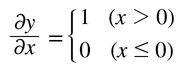
순전파 때의 입력인 x가 0보다 크면 역전파는 상류의 값을 그대로 하류로 흘림.
반면, 순전파 때 x가 0이하면 ㅇ역전파 때는 하류로 신호를 보내지 않음.(0을 보냄)
ReLU 계층의 계산 그래프

# ReLU 계층 구현
class Relu:
  def __init__(self):
    self.mask = None

  def forward(self, x):
    self.mask = (x <= 0)
    out = x.copy()
    out[self.mask] = 0

    return out

  def backward(self, dout):
    dout[self.mask] = 0
    dx = dout

    return x
import numpy as np
x = np.array( [[1.0, -0.5], [-2.0, 3.0]])
print(x)
mask = (x <= 0)
print(mask)>>> [[ 1. -0.5]
[-2. 3. ]]
[[False True]
[ True False]]
- Sigmoid 계층
Sigmoid 계층의 계산 그래프(순전파)

Sigmoid 함수 역전파


위의 과정을 모두 묶어 sigmoid 노드 하나로 대체 가능

# Sigmoid 구현

class Sigmoid:
  def __init__(self):
    self.out = None

  def forward(self, x):
    out = 1 / (1 + np.exp(-x))
    self.out = out

    return out

  def backward(self, dout):
    dx = dout * (1.0 - self.out) * self.out

    return dx
- Affine/Softmax 계층 구현하기
Affine 계층
: 신경망의 순전파 때 수행하는 행렬의 곱은 기하학에서 어파인변환(Affine transformation)이라고 함.
X, W, B의 행렬 흐름

배치용 Affine 계층

# 배치용 Affine 계층 구체적인 예
X_dot_W = np.array([[0,0,0],[10,10,10]])
B = np.array([1,2,3])
print(X_dot_W)
print(X_dot_W + B)
>>> [[ 0 0 0]
[10 10 10]]
[[ 1 2 3]
[11 12 13]]
# 순전파의 편향 덧셈은 각각의 데이터에 더해짐.
# 역전파 때는 각 데이터의 역전파 값이 편향의 원소에 모여야 함.

dY = np.array([[1,2,3],[4,5,6]])
print(dY)
dB = np.sum(dY, axis = 0)
print(dB)
>>> [[1 2 3]
[4 5 6]]
[5 7 9]
# Affine 구현
class Affine:
  def __init__(self, W, b):
    self.W = W
    self.b = b
    self.x = None
    self.dW = None
    self.db = None

  def forward(self, x):
    self.x = x
    out = np.dot(x, self.W) + self.b

    return out

  def backward(self, dout):
    dx = np.dot(dout, self.W.T)
    self.dW = np.dot(self.x.T, dout)
    self.db = np.sum(dout, axis = 0)

    return dx
- Softmax-with-Loss 계층
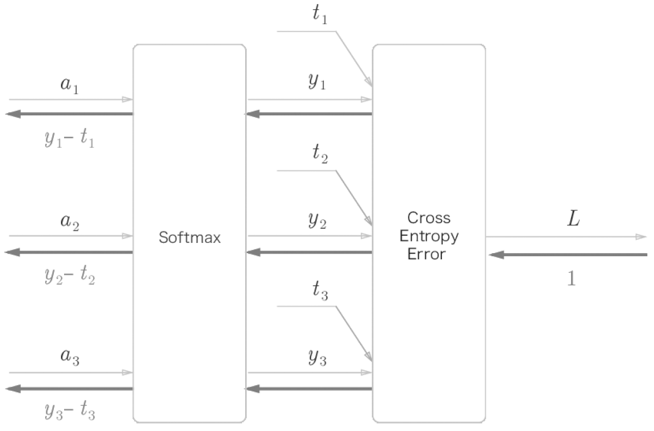
Softmax 함수는 입력 값을 정규화하여 출력함.

손실 함수인 교차 엔트로피(cross-entropy)오차도 포함하여 'Softmax-with-Loss계층'이라는 이름으로 구현함.
Softmax-with-Loss 계층의 계산 그래프

간소화한 Softmax-with-Loss 계층의 계산 그래프
# Softmax-with-Loss 계층 구현
class SoftmaxWithLoss:
  def __init__(self):
    self.loss = None  # 손실
    self.y = None     # softmax의 출력
    self.t = None     # 정답 레이블(원-핫 벡터)

  def forward(self, x, t):
    self.t = t
    self.y = softmax(x)
    self.loss = corss_entropy_error(self.y, self.t)
    return self.loss

  def backward(self, dout=1):
    batch_size = self.t.shape[0]
    dx = (self.y - self.t) / batch_size

    return dx
참고: 밑바닥부터 시작하는 딥러닝 1
notebook ipynb file: https://github.com/heejvely/Deep_learning/blob/main/%EB%B0%91%EB%B0%94%EB%8B%A5%EB%B6%80%ED%84%B0_%EC%8B%9C%EC%9E%91%ED%95%98%EB%8A%94_%EB%94%A5%EB%9F%AC%EB%8B%9D_1/%EC%98%A4%EC%B0%A8%EC%97%AD%EC%A0%84%ED%8C%8C%EB%B2%95.ipynb
GitHub - heejvely/Deep_learning: deep learning 기초 공부
deep learning 기초 공부. Contribute to heejvely/Deep_learning development by creating an account on GitHub.
github.com
'Deep Learning' 카테고리의 다른 글
| [Deep Learning] 가중치의 초깃값 (0) | 2022.11.13 |
|---|---|
| [Deep Learning]Optimizer 매개변수 갱신 (2) | 2022.11.13 |
| [Deep Learning]오차역전파의 계산법 (0) | 2022.11.11 |
| [Deep Learning]최소제곱법 (0) | 2022.11.10 |
| [Deep Learning] 오차역전파법 구현(Back Propagation) (0) | 2022.11.07 |