이전 deep learning 클래스 코드 구현과 이어지는 내용이므로, 이전 글 먼저 확인하는 것이 좋습니다.
https://heejins.tistory.com/36
[Deep Learning] 딥러닝 클래스 코드 구현(연산, layer, neuralnetwork, 배치학습, optimizer)
import numpy as np from numpy import ndarray from typing import * def assert_same_shape(array: ndarray, array_grad: ndarray): assert array.shape == array_grad.shape, \ f""" 두 ndarray의 모양이 같아야 하는데, 첫 번째 ndarray의 모양은 {tupl
heejins.tistory.com
- 소프트맥스 교차 엔트로피 손실 함수(SofrmaxCrossEntropyLoss)
class SoftmaxCrossEntropyLoss(Loss):
  def __init__(self, eps: float = 1e-9):
    super().__init__()
    self.eps = eps
    self.single_output = False

  def _output(self) -> float:

    # 각 행(관찰에 해당)에 softmax 함수 적용
    softmax_preds = softmax(self.prediction, axis = 1)

    # 손실값이 불안정해지는 것을 막기 위해 softmax 함수의 출력값 범위를 제한
    self.softmax_preds = np.clip(softmax_preds, self.eps, 1 - self.eps)

    # 실제 손실값 계산 수행
    softmax_cross_entropy_loss = (
        -1.0 * self.target * np.log(self.softmax_preds) - (1.0 - self.target) * np.log(1 - self.softmax_preds)
    )

    return np.sum(softmax_cross_entropy_loss)

  def _input_grad(self) -> ndarray:
    return self.softmax_preds - self.target
활성화 함수 선택하기
sigmoid 함수가 활성화 함수로 적합한 이유
- 단조함수이며 비선형 함수다.
- 중간 특징의 값을 유한한 구간으로 제한(특히 [0,1] 구간)해서 모델에 제약을 건다.
sigmoid 함수 단점
- 기울기가 상대적으로 평탄해서 역방향 계산에 불리함.
- sigmoid 함수의 최대 기울기는 0.25이므로 연산 한 단계를 통과할 때마다 기울기 값이 ¼로 줄어듦.
- 그래프가 x = -2나 x = 2일 때 거의 평탄해 지므로 -2보다 작거나 2보다 크면 이때 기울기는 0에 가까워짐.
Sigmoid 함수
def sigmoid(x):
    return 1 / (1 + np.exp(-x))


a = np.arange(-5, 5, 0.01)
plt.plot(a, sigmoid(a))
plt.title("Sigmoid 함수")
plt.xlabel("$x$")
plt.ylabel("$Sigmoid(x)$");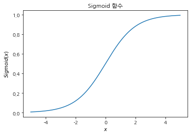
ReLU 함수
def relu(x):
    return np.array([el if el > 0 else 0 for el in x])

a = np.arange(-5, 5, 0.01)
plt.plot(a, relu(a))
plt.title("ReLU 활성화 함수")
plt.xlabel("X")
plt.ylabel("$ReLU(x)$");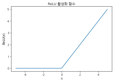
Tanh 함수
a = np.arange(-5, 5, 0.01)
plt.plot(a, np.tanh(a))
plt.title("Tanh 활성화 함수")
plt.xlabel("$x$")
plt.ylabel("$Tanh(x)$")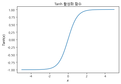
Sigmoid와 Tanh 두 함숨의 기울기 변화 그래프
a = np.arange(-5, 5, 0.01)
plt.figure(figsize = (8,6))
plt.plot(a, sigmoid(a) * (1 - (sigmoid(a))))
plt.plot(a, 1 - (np.tanh(a) ** 2))
plt.legend(['$sigmoid(x)$의 도함수',
            '$Tanh(x)$의 도함수'])
plt.title("$sigmoid(x)$와 $Tanh(x)$의 도함수")
plt.xlabel("x")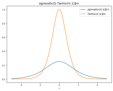
→ Sigmoid는 최대 0.3 정도로, vanishing gradient(기울기 손실) 문제가 발생할 수 있음.
- mnist data로 모델 학습 진행 및 평가
lincoln 라이브러리 임포트
import lincoln
from lincoln.layers import Dense
from lincoln.losses import SoftmaxCrossEntropy, MeanSquaredError
from lincoln.optimizers import Optimizer, SGD, SGDMomentum
from lincoln.activations import Sigmoid, Tanh, Linear, ReLU
from lincoln.network import NeuralNetwork
from lincoln.train import Trainer
from lincoln.utils import mnist
from lincoln.utils.np_utils import softmax
data load
# 데이터 로드
X_train, y_train, X_test, y_test = mnist.load()
num_labels = len(y_train)
num_labels60000data preprocessing
# 원 핫 인코딩
num_labels = len(y_train)
train_labels = np.zeros((num_labels, 10))
for i in range(num_labels):
  train_labels[i][y_train[i]] = 1

num_labels_test = len(y_test)
test_labels = np.zeros((num_labels_test, 10))
for i in range(num_labels_test):
  test_labels[i][y_test[i]] = 1
데이터를 평균 0, 분산 1로 정규화
X_train, X_test = X_train - np.mean(X_train), X_test - np.mean(X_train)np.min(X_train), np.max(X_train), np.min(X_test), np.max(X_test)(-33.318421449829934,
221.68157855017006,
-33.318421449829934,
221.68157855017006)X_train, X_test = X_train / np.std(X_train), X_test / np.std(X_train)np.min(X_train), np.max(X_train), np.min(X_test), np.max(X_test)(-0.424073894391566, 2.821543345689335, -0.424073894391566, 2.821543345689335) def calc_accuracy_model(model, test_set):
return print(f'''모델 검증을 위한 정확도: {np.equal(np.argmax(model.forward(test_set, inference=True), axis=1), y_test).sum() * 100.0 / test_set.shape[0]:.2f}%''')모델
소프트맥스 교차 엔트로피 손실함수 실험 - sigmoid 활성화 함수를 사용, MeanSquaredError 손실함수 사용한 경우
model = NeuralNetwork(layers = [Dense(neurons = 89,
                                      activation = Tanh()),
                                Dense(neurons = 10,
                                      activation = Sigmoid())],
                      loss = MeanSquaredError(),
                      seed = 20190119)

optimizer = SGD(0.1)

trainer = Trainer(model, optimizer)
trainer.fit(X_train, train_labels, X_test, test_labels,
            epochs = 50,
            eval_every = 10,
            seed = 20190119,
            batch_size = 60)

calc_accuracy_model(model, X_test)
10에폭에서 검증 데이터에 대한 손실값: 0.611
20에폭에서 검증 데이터에 대한 손실값: 0.427
30에폭에서 검증 데이터에 대한 손실값: 0.389
40에폭에서 검증 데이터에 대한 손실값: 0.373
50에폭에서 검증 데이터에 대한 손실값: 0.365
모델 검증을 위한 정확도: 72.67%같은 조건, normalize True한 경우
model = NeuralNetwork(layers = [Dense(neurons = 89,
                                      activation = Tanh()),
                                Dense(neurons = 10,
                                      activation = Sigmoid())],
                      loss = MeanSquaredError(normalize=True),
                      seed = 20190119)

optimizer = SGD(0.1)

trainer = Trainer(model, optimizer)
trainer.fit(X_train, train_labels, X_test, test_labels,
            epochs = 50,
            eval_every = 10,
            seed = 20190119,
            batch_size = 60)

calc_accuracy_model(model, X_test)
10에폭에서 검증 데이터에 대한 손실값: 0.952
20에폭에서 손실값이 증가했다. 마지막으로 측정한 손실값은 10 에폭까지 학습된 모델에서 계산된 0.952이다.
모델 검증을 위한 정확도: 41.73%소프트맥스 교차 엔트로피 손실함수 실험 - Linear 활성화 함수를 사용, SoftmaxCrossEntropy 손실함수 사용한 경우
model = NeuralNetwork(layers = [Dense(neurons = 89,
                                      activation = Tanh()),
                                Dense(neurons = 10,
                                      activation = Linear())],
                      loss = SoftmaxCrossEntropy(),
                      seed = 20190119)

optimizer = SGD(0.1)

trainer = Trainer(model, optimizer)
trainer.fit(X_train, train_labels, X_test, test_labels,
            epochs = 50,
            eval_every = 10,
            seed = 20190119,
            batch_size = 60)

calc_accuracy_model(model, X_test)
10에폭에서 검증 데이터에 대한 손실값: 0.619
20에폭에서 검증 데이터에 대한 손실값: 0.568
30에폭에서 검증 데이터에 대한 손실값: 0.548
40에폭에서 검증 데이터에 대한 손실값: 0.548
50에폭에서 검증 데이터에 대한 손실값: 0.547
모델 검증을 위한 정확도: 90.95%ReLU 활성화 함수를 사용한 경우
model = NeuralNetwork(
    layers=[Dense(neurons=89,
                  activation=ReLU()),
            Dense(neurons=10,
                  activation=Linear())],
            loss = SoftmaxCrossEntropy(),
seed=20190119)

trainer = Trainer(model, SGD(0.1))
trainer.fit(X_train, train_labels, X_test, test_labels,
            epochs = 50,
            eval_every = 10,
            seed=20190119,
            batch_size=60);
print()
calc_accuracy_model(model, X_test)
10에폭에서 검증 데이터에 대한 손실값: 7.474
20에폭에서 손실값이 증가했다. 마지막으로 측정한 손실값은 10 에폭까지 학습된 모델에서 계산된 7.474이다.
모델 검증을 위한 정확도: 71.34%model = NeuralNetwork(
layers=[Dense(neurons=89,
activation=Tanh()),
Dense(neurons=10,
activation=Linear())],
loss = SoftmaxCrossEntropy(),
seed=20190119)
trainer = Trainer(model, SGD(0.1))
trainer.fit(X_train, train_labels, X_test, test_labels,
epochs = 50,
eval_every = 10,
seed=20190119,
batch_size=60);
print()10에폭에서 검증 데이터에 대한 손실값: 0.619
20에폭에서 검증 데이터에 대한 손실값: 0.568
30에폭에서 검증 데이터에 대한 손실값: 0.548
40에폭에서 검증 데이터에 대한 손실값: 0.548
50에폭에서 검증 데이터에 대한 손실값: 0.547- 모멘텀
Optimizer 클래스에 모멘텀 구현하기
파라미터 수정에 모멘텀을 적용하면 그때까지 수정했던 파라미터의 각 수정 폭을 시간이 지남에 따라 지수적으로 감쇠하는 가중치로 가중한 평균값을 파라미터 수정 폭으로 삼는다.
따라서 수정 폭의 가중치가 감쇠되는 정도를 결정하는 모멘텀 파라미터가 추가된다. 모멘텀 파라미터의 값이 클수록 현재 속도보다 누적된 파라미터 수정 폭에 더 영향을 많이 받는다.
코드
- Optimizer 클래스에 파라미터를 수정할 때마다 수정 이력 저장
- 그 후 현재 기울기와 이미 저장해둔 수정 이력을 사용하면 실제 파라미터 수정 폭 계산 가능
- 모멘텀이 물리학에서 차용한 개념인 만큼 이 수정 이력을 속력이라고 부름
[ 속력을 최신 상태로 유지하는 방법 ]
- 모멘텀 파라미터를 곱한다
- 현재 기울기를 더한다.
SGDMomentum 클래스
class SGDMomentum(Optimizer):
  """
  확률적 경사 하강법을 적용한 Optimizer
  """
  def __init__(self,
               lr: float = 0.01,
               momentum: float = 0.9) -> None:
    super().__init__()
    self.lr = lr
    self.momentum = momentum

  def step(self):
    """
    첫 번째 반복인 경우 각 파라미터의 속력을 초기화한다.
    첫 번째 반복이 아니라면 _update_rule을 적용한다.
    """
    if self.first:
      # 첫 번째 반복에서 속력 초기화
      self.velocities = [np.zeros_like(param) for param in self.net.params()]
      self.first = False


    for (param, param_grad, velocity) in zip(self.net.params(),
                                   self.net.param_grads(),
                                   self.velocities):
      # _update_rule 메서드에 속력 전달
      self._update_rule(param = param,
                        grad = param_grad,
                        velocity = velocity)

  def _update_rule(self, ** kwargs) -> None:
    """
    모멘텀을 적용한 파라미터 수정 규칙
    """
    # 속력 업데이트
    kwargs['velocity'] *= self.momentum
    kwargs['velocity'] += self.lr * kwargs['grad']

    # 파라미터 수정에 속력을 포함함
    kwargs['param'] -= kwargs['velocity']
모멘텀을 적용한 확률적 경사 하강법
model = NeuralNetwork(
    layers=[Dense(neurons=89,
                  activation=Sigmoid()),
            Dense(neurons=10,
                  activation=Linear())],
            loss = SoftmaxCrossEntropy(),
seed=20190119)

optim = SGDMomentum(0.1, momentum=0.9)

trainer = Trainer(model, SGDMomentum(0.1, momentum=0.9))
trainer.fit(X_train, train_labels, X_test, test_labels,
            epochs = 50,
            eval_every = 1,
            seed=20190119,
            batch_size=60);

calc_accuracy_model(model, X_test)
1에폭에서 검증 데이터에 대한 손실값: 0.615
2에폭에서 검증 데이터에 대한 손실값: 0.489
3에폭에서 검증 데이터에 대한 손실값: 0.446
4에폭에서 손실값이 증가했다. 마지막으로 측정한 손실값은 3 에폭까지 학습된 모델에서 계산된 0.446이다.
모델 검증을 위한 정확도: 92.13%- 학습률 감쇠(Learning rate decay)
선형 감쇠
model = NeuralNetwork(
    layers=[Dense(neurons=89,
                  activation=Tanh()),
            Dense(neurons=10,
                  activation=Linear())],
            loss = SoftmaxCrossEntropy(),
seed=20190119)

optimizer = SGDMomentum(0.15, momentum=0.9, final_lr = 0.05, decay_type='linear')

trainer = Trainer(model, optimizer)
trainer.fit(X_train, train_labels, X_test, test_labels,
            epochs = 50,
            eval_every = 10,
            seed=20190119,
            batch_size=60);

calc_accuracy_model(model, X_test)
0에폭에서 검증 데이터에 대한 손실값: 0.380
20에폭에서 검증 데이터에 대한 손실값: 0.321
30에폭에서 검증 데이터에 대한 손실값: 0.303
40에폭에서 검증 데이터에 대한 손실값: 0.295
50에폭에서 손실값이 증가했다. 마지막으로 측정한 손실값은 40 에폭까지 학습된 모델에서 계산된 0.295이다.
모델 검증을 위한 정확도: 96.06%지수 감쇠
model = NeuralNetwork(
    layers=[Dense(neurons=89,
                  activation=Tanh()),
            Dense(neurons=10,
                  activation=Linear())],
            loss = SoftmaxCrossEntropy(),
seed=20190119)

optimizer = SGDMomentum(0.2,
                        momentum=0.9,
                        final_lr = 0.05,
                        decay_type='exponential')

trainer = Trainer(model, optimizer)
trainer.fit(X_train, train_labels, X_test, test_labels,
            epochs = 50,
            eval_every = 10,
            seed=20190119,
            batch_size=60);

calc_accuracy_model(model, X_test)
10에폭에서 검증 데이터에 대한 손실값: 0.445
20에폭에서 검증 데이터에 대한 손실값: 0.346
30에폭에서 검증 데이터에 대한 손실값: 0.306
40에폭에서 손실값이 증가했다. 마지막으로 측정한 손실값은 30 에폭까지 학습된 모델에서 계산된 0.306이다.
모델 검증을 위한 정확도: 96.05%- 초기 가중치 설정
n_feat = 784
n_hidden = 256

np.random.seed(190131)

a = np.random.randn(1, n_feat)
b = np.random.randn(n_feat, n_hidden)
out = np.dot(a, b).reshape(n_hidden)
fig, ax = plt.subplots(1, 2, figsize=(12, 5))
ax[0].hist(out)
ax[0].set_title("784개 입력을 받는 은닉층의\n 활성화 함수 통과 전 가중합의 분포")
ax[1].hist(np.tanh(out))
ax[1].set_title("784개 입력을 받는 은닉층의\n tanh 활성화 함수를 통과한 출력값의 분포")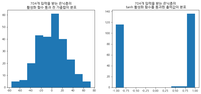
선형감쇠(early_stopping = True arg 추가)
model = NeuralNetwork(
    layers=[Dense(neurons=89,
                  activation=Tanh(),
                  weight_init="glorot"),        # glorot 초기화 이용
            Dense(neurons=10,
                  activation=Linear(),
                  weight_init="glorot")],
            loss = SoftmaxCrossEntropy(),
seed=20190119)

optimizer = SGDMomentum(0.15, momentum=0.9, final_lr = 0.05, decay_type='linear')

trainer = Trainer(model, optimizer)
trainer.fit(X_train, train_labels, X_test, test_labels,
       epochs = 50,
       eval_every = 10,
       seed=20190119,
           batch_size=60,
           early_stopping=True);

calc_accuracy_model(model, X_test)
10에폭에서 검증 데이터에 대한 손실값: 0.377
20에폭에서 검증 데이터에 대한 손실값: 0.260
30에폭에서 검증 데이터에 대한 손실값: 0.222
40에폭에서 손실값이 증가했다. 마지막으로 측정한 손실값은 30 에폭까지 학습된 모델에서 계산된 0.222이다.
모델 검증을 위한 정확도: 97.04%지수감쇠(early_stopping = True arg 추가)
model = NeuralNetwork(
    layers=[Dense(neurons=89,
                  activation=Tanh(),
                  weight_init="glorot"),
            Dense(neurons=10,
                  activation=Linear(),
                  weight_init="glorot")],
            loss = SoftmaxCrossEntropy(),
seed=20190119)

trainer = Trainer(model, SGDMomentum(0.15, momentum=0.9, final_lr = 0.05, decay_type='exponential'))
trainer.fit(X_train, train_labels, X_test, test_labels,
       epochs = 50,
       eval_every = 10,
       seed=20190119,
           batch_size=60,
           early_stopping=True);

calc_accuracy_model(model, X_test)
10에폭에서 검증 데이터에 대한 손실값: 0.295
20에폭에서 검증 데이터에 대한 손실값: 0.223
30에폭에서 손실값이 증가했다. 마지막으로 측정한 손실값은 20 에폭까지 학습된 모델에서 계산된 0.223이다.
모델 검증을 위한 정확도: 96.62%- 드롭아웃(Dropout)
드롭아웃을 적용하면 과적합을 일으키지 않으면서도 더 복잡한 모델을 학습 할 수 있다.
class Dropout(Operation):
  def __init__(self,
               keep_prob: float = 0.8):
    super().__init__()
    self.keep_prob = keep_prob

  def _output(self, inference: bool) -> ndarray:
    if inference:
      return self.inputs * self.keep_prob
    else:
      self.mask = np.random.binomial(1, self.keep_prob,
                                     size = self.inputs.shape)
      return self.inputs * self.mask

  def _input_grad(self, output_grad: ndarray) -> ndarray:
    return output_grad * self.mask
드롭아웃을 적용하기 위해 프레임워크 수정하기
- Layer와 NeuralNetwork 클래스의 forward 메서드에 인자 inference를 추가하고(기본값은 False) 이 플래그의 값을 그대로 각 Operation에 전달해서 Operation 클래스가 추론 모드와 학습 모드로 나뉘어 동작할 수 있도록 한다.
- Trainer 클래스에서 학습 중 eval_every 에폭마다 그 시점까지 학습된 모델을 테스트하는 부분에 inference 플래그를 True로 설정한다.
- 마지막으로 Layer 클래스의 생성자 메서드에 dropout 이라는 키워드 인자를 추가한다. 수정된 Layer 클래스의 생성자 메서드는 다음과 같은 시그니처를 갖는다.
def __init__(self, neurons: int, activation:Operation = Linear(), dropout: float = 1.0, weight_init: str = 'standard') - 그리고 _setup_layer 메서드에서 다음과 같이 마지막 연산으로 dropout 연산을 추가한다.
if self.dropout < 1.0:
self.operations.append(Dropout(self.dropout))드롭아웃 실험
mnist_soft = NeuralNetwork(
    layers = [Dense(neurons = 89,
                    activation = Tanh(),
                    weight_init = 'glorot',
                    dropout = 0.8),
              Dense(neurons = 10,
                    activation = Linear(),
                    weight_init = 'glorot')],
              loss = SoftmaxCrossEntropy(),
              seed = 20190119
)

trainer = Trainer(model, SGDMomentum(0.2, momentum=0.9, final_lr = 0.05, decay_type='exponential'))
trainer.fit(X_train, train_labels, X_test, test_labels,
       epochs = 100,
       eval_every = 10,
       seed=20190119,
           batch_size=60,
           early_stopping=True);

calc_accuracy_model(model, X_test)
10에폭에서 검증 데이터에 대한 손실값: 0.441
20에폭에서 검증 데이터에 대한 손실값: 0.349
30에폭에서 검증 데이터에 대한 손실값: 0.268
40에폭에서 검증 데이터에 대한 손실값: 0.250
50에폭에서 손실값이 증가했다. 마지막으로 측정한 손실값은 40 에폭까지 학습된 모델에서 계산된 0.250이다.
모델 검증을 위한 정확도: 96.40%은닉층의 뉴런 수를 두배로 늘리고(178), 두 번째 은닉층은 기존 첫 번째 은닉층 뉴런 수의 절반 정도(46)로 설정한다.
mnist_soft = NeuralNetwork(
    layers = [Dense(neurons = 178,
                    activation = Tanh(),
                    weight_init = 'glorot',
                    dropout = 0.8),
              Dense(neurons = 46,
                    activation = Tanh(),
                    weight_init = 'glorot',
                    dropout = 0.8),
              Dense(neurons = 10,
                    activation = Linear(),
                    weight_init = 'glorot')],
              loss = SoftmaxCrossEntropy(),
              seed = 20190119
)

trainer = Trainer(model, SGDMomentum(0.2, momentum=0.9, final_lr = 0.05, decay_type='exponential'))
trainer.fit(X_train, train_labels, X_test, test_labels,
       epochs = 100,
       eval_every = 10,
       seed=20190119,
           batch_size=60,
           early_stopping=True);

calc_accuracy_model(model, X_test)
10에폭에서 검증 데이터에 대한 손실값: 0.441
20에폭에서 검증 데이터에 대한 손실값: 0.349
30에폭에서 검증 데이터에 대한 손실값: 0.268
40에폭에서 검증 데이터에 대한 손실값: 0.250
50에폭에서 손실값이 증가했다. 마지막으로 측정한 손실값은 40 에폭까지 학습된 모델에서 계산된 0.250이다.
모델 검증을 위한 정확도: 96.40%
- 출처: 처음 시작하는 딥러닝
- notebook ipynb file: https://github.com/heejvely/Deep_learning/blob/main/%EC%B2%98%EC%9D%8C_%EC%8B%9C%EC%9E%91%ED%95%98%EB%8A%94_%EB%94%A5%EB%9F%AC%EB%8B%9D/%ED%94%84%EB%A0%88%EC%9E%84%EC%9B%8C%ED%81%AC%20%ED%99%95%EC%9E%A5%ED%95%98%EA%B8%B0.ipynb
GitHub - heejvely/Deep_learning: deep learning 기초 공부
deep learning 기초 공부. Contribute to heejvely/Deep_learning development by creating an account on GitHub.
github.com
'Deep Learning' 카테고리의 다른 글
| [Deep Learning] 순환 신경망(RNN) (0) | 2023.01.08 |
|---|---|
| [Deep Learning] 모델 설계하기 (0) | 2022.12.30 |
| [Deep Learning] 딥러닝 클래스 코드 구현(연산, layer, neuralnetwork, 배치학습, optimizer) (0) | 2022.11.23 |
| [Deep Learning] 오차 수정하기: 경사하강법, 편미분 코드 구현 (0) | 2022.11.22 |
| [Deep Learning]퍼셉트론(Perceptron) (0) | 2022.11.16 |